Grasping transient phenomena #

Interesting phenomena are, almost by definition, rare. Think of the perfect investment opportunity, a marriage, a stock market crash, an epidemic, a cure, societal change, and so forth. In a sense their ‘interesting-ness’ is derived from the fact that they are in contrast to every day, average observations. They are also transient, in that they occur once and rarely repeat, if they repeat they usually differ markedly. For example, few stock market crashes are identical, and not a daily occurrence. Nicholas Taleb in his books, leading with the ‘Black Swan’, makes a similar point. He also mentions that common models used in analysis do not care about rare or transient events, but do care about the average. A key example is the Normal distribution. If your data has extreme events, any fit of a Normal distribution will indeed match the majority of the data quite well, but have an increasingly larger error just where you do not want it, in the tails or the extreme values. This does not mean the Normal distribution is a ‘bad’ model, just that you should be very careful when and where to use it. If indeed all you care about it the average event, then your choice is indeed a good one.

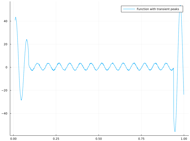
Let’s look at an example of a continuous, noisy, oscillating function, with 2 transient events (~ spikes).

Approximation functions as models #

Being able to detect, locate, quantify, and predict transient events is therefore of extreme value. If we abstract away any of our ’events’ as a numerical sequence S, , occurring over time, then we can formulate ways to approximate this series of numbers with a function f. Once we have f we can interpret patterns, quantify, predict and so forth, within the limits of the approximation. A bit more formally

\(S: t \rightarrow \mathbb{R}\)

\(f: t \rightarrow \mathbb{R}\)

\(\vert \vert S(t), f(t) \vert \vert \leq \epsilon, ~ \forall t \in T, \exists ϵ \in \mathbb{R}, \epsilon \leq \infty\)

Essentially we want the error between our approximation (model) f and the sequence to be finite and small.

The dangers of perfection #

Beware, however, you may want to think that it’s a good feature if your chosen f has an ϵ of 0. It’s not. Essentially what you now have done is replaced your function, or model, with your data. The reason why this is unwanted is that your data is not actually your true data or information, it’s an observation occluded by a lot of noise. There’s measurement noise, because there’s no such thing as infinite precision, there’s selection noise, where you capture data you wish to see, and more likely than not your data has confounding and correlated variables that are either present, or unmeasured. So in reality our information I is

\(I: t \rightarrow \mathbb{R}\)

measured by our signal S

\(S: t \rightarrow \mathbb{R}\)

such that

\(S = \theta(\gamma(I) + \delta) \)

Here δ is additive noise, the simplest form. Gamma can be seen as perceptional noise, a black box function that attempts to see I through its own lens, and θ can represent another function representing our measurement skew. There are many different models of information and noise, my example here is by no means complete or unique. To illustrate why I didn’t just keep it to additive noise, let the information be the light of a cluster of stars. δ could be the light of a street lamp masking fainter stars. γ can be a black hole on the path between you and the star, warping the photon path. Θ, finally, can be the optical effects of an imperfect lens you’re using in your telescope. You can come up with more levels of noise, but it should be clear by now that there’s a huge gap between information and signal, so equating both is not a good thing (tm).

We are interested not in S, but in I. So if f == S, or ϵ=0, then we’re essentially conditioning perfectly on noise. In some contexts this can be identified with overfitting, but not entirely. Overfitting, in my interpretation, can also occur if you fit a model perfectly on seen data, in such a way that you now have an unbounded error on unseen data. Minimizing ϵ to 0 is not the same.

Suppose we come up with a model that fits all stock exchange data perfectly up until 1928. We haven’t used 1929, the infamous crash introducing the Depression, as data yet. Our model can now perfectly predict any data point < 1929. However, it’s useless in 1929, because it will not protect us from more than a decade of misery. Here we overfitted, but our error is not zero, in fact, in 1929 you may as well express the error in societal terms as ‘worst ever’.

An example of ϵ = 0 is essentially replacing your model with your data. And when I now ask you to interpret, or see patterns, in you model (which is your data), you’d come back with the same answer every time : your data. Your model, or approximation is only useful if it diverges from your data, but only diverges is a predictable, limited way. For example, say the best model f you find, with a limited error, is the sine function.

\(f(t) = b \sin(t + a) \)

Now you define the period, magnitude, and so on of this function. In real world data, you’d be able to predict events because they’re periodic, and with some error you’d be able to predict their magnitude.

If your data is actually a sine function, then there’d be no point in analyzing it in the first place by a model or approximation.

The dangers of averaging approximation. #

A key tool in function approximation is the Fourier series:

\(f(x) = \frac{a_0}{2} + \sum_{k=1}^N(a_k \cos(kx) + b_k \sin(kx)\)

There are, naturally, many more, but I pick Fourier here to make a point. As you can observe, f(x) is a composition of functions (sine, cosine) that have infinite support. Infinite support is best defined in terms of what it is not, limited or finite support.

\( f(x) = 0 \Leftrightarrow x < k \lor x > j, \exist k < j, k, j \in \mathbb{R} \)

In other words, f is zero except in the interval [k,j]. You can see that for sine and cosine k and j are -∞ and +∞, so they do not have finite support.

Another way of saying that f has finite support could be

\( 0 < \int_a^b f(x) < \infty , \exist~ a < b \in \mathbb{R} \)

Finite support matters because if you try to approximate a function by composing infinite support functions, you run into issues, for the Fourier series best illustrated by the Runge phenomenon. Detailing this will take us too far, but think of it this way, if we see the crash of ‘29 as sudden, never-occurred before (or since), spike in the the stock prices, then that’s a transient signal. We now try to ‘glue’ together the stock price function by using sines and cosines, and run into the issue that getting that one spike to fit will introduce errors in other places, because there’s no single composite function that only is active at 1929. Nonetheless, it is known that with Fourier you can approximate a function arbitrarily close, given infinite terms.

\( \lim_{n \rightarrow ∞} f_n(x) - S(x) = 0\)

So how do we reconcile this? Surely we just need ’enough’ terms to make this work?

Not really, by now it should be clear that we’re interested in, well, interesting patterns. Not the average. And yet there the error will converge the slowest.

Second, because sine and cosine have infinite support, the coefficients won’t tell us much about the location of transient or interesting events. If I give you the ai and bi coefficients of a Fourier series approximating the stock price from 1900 to 1990, just by looking at those you can’t tell me when the stock market crashed.

So in addition to finite support, our model really should have location sensitive parameters. In the end, we want to understand the model, and the data through the model.

Why Wavelets function better #

Ideally, our approximation function should have

• finite support components
• coefficients that locate patterns
• fast convergence to (almost 0) error

Before, we used sine and cosine, which are wave functions, they oscillate and without damping continue in perpetuity. A wavelet then, is a damped wave. It’s that simple. In order to work as an approximation function f:

\( f(x) = \sum_{j \in \mathbb{Z}} \sum_{k \in \mathbb{Z}} c_{j,k} \psi_{j,k} (x) \)

where ψ is our wavelet, we need the following to hold:

\( \psi_{j,k}(x) = 2^{j/2}\psi(2^jx - k) \vert j, k \in \mathbb{Z}\)

and \(\langle \psi_{j,k} \psi_{i,l} \rangle = 0, ~~ \forall (i,j) \neq (j,k)\)

If you can find a function ψ, then any finite function on finite support (and the stock exchange is both), can be written as a composition of a recursive scaling (j) and translation (k) of ψ. The difficulty lies in finding such a function.

The last condition essentially states that the composite function are orthogonal.

I’m going to keep details on the finer points of the underlying math for my slidedeck here, and instead focus on a simple example in Julia.

Haar Wavelet #

The Haar Wavelet are piecewise constant functions on [0,1), among the simplest functions you can define. Yet they can form a perfect candidate for ψ:

ϕ(x) =  0 <= x < 1 ? 1 : 0 # Father Wavelet
ψ(x) =  ϕ(2*x) - ϕ(2*x-1) # Mother wavelet

Next, we define the recurrence (or generations), using currying.

ψ(n, k, x) = ψ(2^n * x - k)
ψ(n, k) = x -> ψ(n, k, x)
ϕ(n, k, x) = ϕ(2^n * x - k)   # 0 <= k <= 2^n -1
ϕ(n, k) = x -> ϕ(n, k, x)

Given a signal, we can now find, using linear algebra, the coefficients:

using Random
# Convenience function to transform functions to vectors
▒▒(~) = hcat([f.(xspace) for f in ~]...)'
# 2 generations of wavelets
q = [ϕ, ψ, ψ10, ψ11 ]

Mn = ▒▒(q)
Random.seed!(42)
# Signal
signal = rand(4)
# Find the coefficients  coeff = Vn \ signal
α = Mn' \ signal

And that’s all there is to it.

Let’s plot the first generation of Haar wavelets.

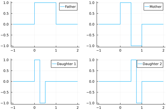
What if you signal > 4 ? You apply the matrix piecewise, for every 4 indices. Or if you prefer a higher resolution, you can create more generations, at a higher computational cost. A more interesting part of Wavelet theory is multi-resolution analaysis, but I will leave that for the slide deck at the end.

Let’s make an example function with some odd transient patterns to see how Wavelet coefficients work

using Plots
n = 4
xspace = 0:1/n:0.9 |> collect
openrange(a, b, step) = a:step:(b-step) |> collect
f(x) = x < 0.09 ? sin(100*x)*(log(x/10))^2 +rand() : (x < 0.94 ? 3*sin(100*x)+rand() : 5*sin(100*(x-0.9))*(log((x-.6)/10))^2 +rand())
u = [ϕ(1,0), ϕ(1,1), ψ(1,0), ψ(1,1)]
xs = openrange(0.01, 1, 0.001);
Plots.plot(xs, f.(xs), label="Function with transient peaks", size=(800,600))  |  

Note the uncharacteristic spikes at left and right ends of the interval. The rest of the function is a noisy sine wave, once you observe its period it’s very predictable. But the two spikes are unexpected, and with very limited support, so hard to approximate when you’d use infinite support functions.

Location aware compression #

We can filter out wavelet coefficients and keep the 90th quantile, to achieve lossy compression. Because our wavelet coefficients are local, we can actually do one better and come up with adaptive compression. Regardless, a transient signal will have a large coefficient, so is unlikely to be filtered out.

First, we show the coefficients when we have 99th quantile, and 90th, as well as non-filtered.

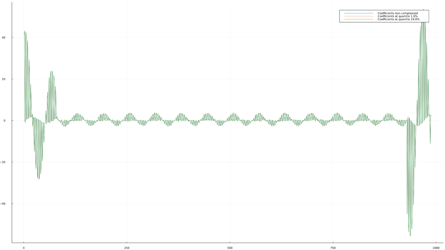
You can see that the coefficients are visually hard to differentiate when compressed, e.g. there seems to be almost no loss. Second, and more importantly, reading the coefficients is almost the same as reading the function. This would not be the case for e.g. Fourier.

Next we show the approximation error

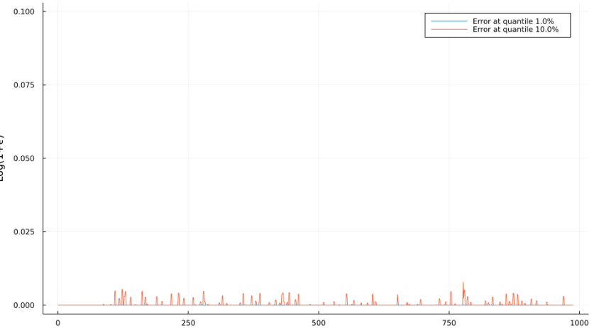
Note how the error is spread out, but by design avoids the ’transient’ parts of the reconstructed function.

Slides #

You can find a presentation of wavelets and current applications here, the slidedeck also covers more of the mathematical background and has references to relevant literature.